Denoising with CNNs, the COVID-19 Detection Case Study

• Introduction
• Ultrasound for COVID-19
  • Why is ultrasound good?
  • Why is ultrasound challenging?
  • What methods are suitable for LUS image denoising?
• Denoising with Deep Image Prior
  • The idea behind DIP
  • Implementation of DIP
    • Testing the performance
    • Examples of denoised data
• Denoising with classical methods
• Classification of LUS images
  • Data pre-processing
  • Building the classifier
  • Does denoising increase the accuracy?
• Conclusions
• References

Introduction

During the COVID-19 pandemic, several methods have been utilized to assist physicians in diagnosing COVID-19.Medical imaging takes a key role in complementing diagnostic tools from molecular biology, and, using deep learning techniques, it's even possible to build automated detection systems. I will be focusing on the lung ultrasound (LUS) imaging, with the goal to improve existing LUS-based detection techniques.

Ultrasound for COVID-19

Why is ultrasound good?

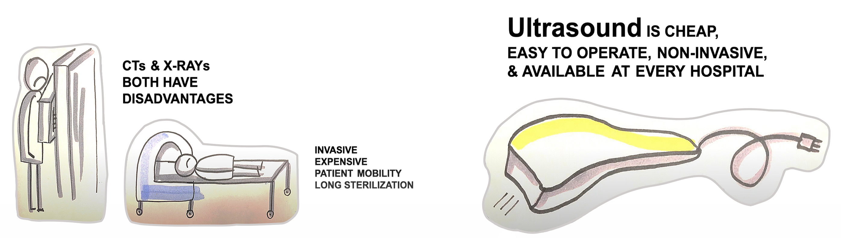
Figure 2.1. Three ways to diagnose COVID-19 via medical imaging [1].

Many voices from the medical community have advocated for a more prominent role of ultrasound for COVID-19 diagnosis [2]. It has several advantages over the alternative imaging modalities, such as CT and X-Ray.

Namely, ultrasound is

• Cheap
• Easy to operate
• Portable, thus suitable for point-of-care use
• Non-invasive and safe
• Fast
• Easy to disinfect
• Available in almost all medical facilities

Moreover, ultrasound data was shown to be highly correlated with CT, the gold standard for lung diseases [3].

Why is ultrasound challenging?

Figure 2.2. Typical LUS patterns. A: COVID-19 infected lung, showing small subpleural consolidation and pleural irregularities. B: Pneumonia infected lung, with dynamic air bronchograms surrounded by alveolar consolidation. C: Healthy lung, normally aerated with horizontal A-lines. [4]

As can bee seen in Figure 2.2, LUS patterns are not so easy to interpret and doing it correctly would require some training and experience. In the current situation of pandemic, the time for extensive training of medical staff is limited though. Therefore, having an automated assistance system for doctors that classifies LUS images is very important. In the past months, several teams from Switzerland, Italy and Israel [4, 5, 6] have been developing such systems with the help of deep learning methods.

But why are LUS images so hard to interpret (for both humans and machines)? One reason for that is the large amount of inherent noise. The ultrasound images are inevitably contaminated by the so called speckle noise during acqisition from tissue backscatter.

Many denoising techniques, utilizing both classical and deep learning based approaches, have been proposed for medical image enhancement. However, to the best of our knowledge, none of the aforementioned teams incorporated denoising in their image pre-processing stage.

Thus, our goal is to find the most suitable denoising technique for LUS images. We believe that better image quality will help both doctors and automated systems to make more accurate diagnoses.

• We will analyze the denoised images and try to see if important trends became more clearly visible to the human eye.
• We will also check if denoising the LUS image dataset can help to increase the accuracy of a CNN-based classifier.

What methods are suitable for LUS image denoising?

In this project, we will be using the publicly available LUS image dataset "POCUS" provided in [7].

Below we will consider several characteristics of this dataset and discuss the compatibility of each characteristic with different denoising techniques.

• Data is contaminated with speckle noise. This type of noise is multiplicative, i.e., we have a convolution of the signal with the noise in the frequency domain. Multiplicative noise is therefore harder to remove than additive noise, which is merely added to the signal in both time and frequency. Both classical (based on various filtering, total variation regularization, wavelet denoising) and CNN-based approaches have been proposed to tackle this problem. While classical methods have to be carefully handcrafted and require manual choice of some parameters, CNNs have the advantage of learning from samples.

• No clean data for reference. Typical CNN-based approaches cast the denoising as a supervised learning problem, where the CNN models are trained to learn a mapping from the noisy patch to the clean patch. Since ultrasound images are inherently noisy, we would need to pre-train the network on some other dataset and use transfer learning. This imposes additional challenge of finding the dataset that is similar enough. However, recently there appeared models that learn to restore images by only looking at noisy data (Noise2Noise [8]).

• Medical data should not be affected by hallucination phenomena. In fact, there is another, possibly even more serious drawback of pre-trained neural networks (including Noise2Noise) in the context of medical image enhancement. Since the reconstruction is based on the information previously learned from other images, it can contain false image features that were not actually present in the input image. This phenomenon is known as hallucination (see Figure 3.1). While sometimes acceptable in case of natural images, it must be avoided at all costs in medical imaging, as it can lead to false diagnoses and thus severely compromise patients' safety. Surprisingy, several novel approaches (Deep Image Prior (DIP) [9], Deep Decoder (DD) [10], SinGAN [11]) show that learning from a large dataset of images is not necessary. Instead, a randomly initialized network can be trained per every image, thus avoiding hallucination.
• Relatively small dataset. In addition to the previous consideration, the lack of training data also favours training from a single image, as in DIP, DD, SinGAN.

Figure 3.1. Hallucination phenomena. Left: Hallucinations in retinal OCT scan reconstructed with pre-trained CNN. The white arrow denotes a hallucinated retinal layer that is anatomically incorrect [12]. Right: Image from Google's DeepDream, where neural network "sees" buildings and animals in the clouds.

The review of the methods as well as our analysis is by no means complete. Ideally, we’d like to write a more comprehensive survey and test and compare several approaches, but this would go beyond the scope of this short project.

At the moment, we decided to focus on Deep Image Prior (DIP). One reason for that is the convolutional nature of DIP which fits the scope of AI-2. It’s also a seminal paper and an intriguing state-of-the-art approach.

Denoising with Deep Image Prior

The idea behind DIP

The word prior refers to some underlying assumption about the image and can be seen as a regularization term in the optimization task. This task can be written as follows,

\begin{equation} \min_{x} E(x;x_0)+R(x), \end{equation}

where $E(x;x_0)$ is a task-dependent data term (MSE for denoising), $x_0$ is a corrupted image, and $R(x)$ is an image prior. E.g., in classical TV denoising algorithm, $R(x)$ corresponds to the total variation of a function (thus, the prior assumes that noisy images have high total variation and minimizing it will result in uniform regions in images).

The idea of DIP is to get rid of the explicit regularization term $R(x)$ and use a randomly initialized CNN to construct the output image $x$. Thus, in a way, the network itself becomes an implicit image prior.

Let $f_\theta(z)$ be a CNN with parameters $\theta$ initialized with a random code vector $z$ (Figure 4.1.a). We'll consider the following optimization task,

\begin{equation} \min_{\theta} E(f_\theta(z);x_0). \end{equation}

Unlike conventional approaches, where we search for the answer in the image space, we'll now search for it in the space of neural network's parameters.

Figure 4.1. Deep Image Prior. a) The authors suggest using a U-Net type "hourglass" architecture with skip-connections, where $z$ and $x$ have the same spatial size. The U-Net’s weights are optimized using gradient descent. b) Image space visualization. Often the optimization path will pass close to $x_{gt}$ – the ground truth, and an early stopping (here at time $t_3$) will recover good solution [9].

But why should this work for denoising? At first glance, this makes absolutely no sense. Deep neural networks are powerful enough to memorize the entire image and are likely to give the original noisy image back. However, in [9] the authors show that when we optimize using gradient descent, CNNs "resist" noisy images, and have a bias towards producing clear images. Figure 4.2 provides evidence to support this claim. In addition, Figure 4.1.b suggests that the optimization trajectory passes near good-looking local optimum even if eventually overfitting to noise.

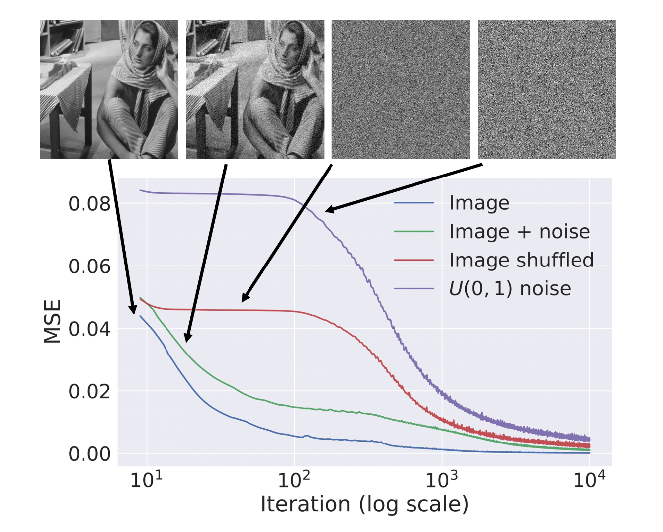
Figure 4.2. Learning curves for optimization of different images. The more noise there is, the slower the loss converges [9].

Implementation of DIP

In their original experiments, the authors used a U-Net type "hourglass" architecture with skip-connections and implemented it in PyTorch. Later there appeared several simplified and computationally less expensive Keras-based implementations (e.g. [13]). We will start with such an implementation utilizing a simple encoder-decoder network and use it as a proof-of-concept for LUS image denoising.

# Define DIP model architecture

def deep_image_prior_model():

    encoding_size = 256

    encoder = Sequential([
        Convolution2D(32, 3, padding='same', input_shape=[256,256,3], activation='relu'),
        Convolution2D(632, 3, padding='same', activation='relu'),
        AveragePooling2D(),
        Convolution2D(64, 3, padding='same', activation='relu'),
        Convolution2D(64, 3, padding='same', activation='relu'),   
        AveragePooling2D(),
        Convolution2D(128, 3, padding='same', activation='relu'),
        Convolution2D(128, 3, padding='same', activation='relu'),
        Flatten(),
        Dense(encoding_size, activation='tanh')
    ])

    decoder = Sequential([
        Dense(768, input_shape=(encoding_size,), activation='relu'),
        Reshape((16, 16, 3)),
        Convolution2D(128, 3, padding='same', activation='relu'),
        Convolution2D(128, 3, padding='same', activation='relu'),
        UpSampling2D(),
        Convolution2D(64, 3, padding='same', activation='relu'),
        Convolution2D(64, 3, padding='same', activation='relu'),
        UpSampling2D(),
        Convolution2D(32, 3, padding='same', activation='relu'),
        Convolution2D(32, 3, padding='same', activation='relu'),
        UpSampling2D(),    
        Convolution2D(16, 3, padding='same', activation='relu'),
        Convolution2D(16, 3, padding='same', activation='relu'),
        UpSampling2D(),
        Convolution2D(8, 3, padding='same', activation='relu'),
        Convolution2D(3, 3, padding='same', activation='tanh')
    ])

    autoencoder = Sequential([
        encoder, 
        decoder
    ])
    
    autoencoder.compile(loss='mse', optimizer=Adam(lr=0.0001))
    return autoencoder

Testing the performance

In order to be able to quantify the performance, we need to test the network on a pair of ground truth and noisy images. Since there is no ground truth for LUS images, we've artificially created an image which looks similar to LUS but is smooth, and contaminated it with the speckle noise taken from real data.

# Define funtions to change pixel range between [0, 255] and [-1, 1]

def normalize(image):            
  return (image/255 - 0.5)*2
def to_image(normalized_image):  
  return ((normalized_image/2 + 0.5) * 255).astype(np.uint8)

# Load images

im = cv2.imread("/content/drive/My Drive/ai2_project/test_0.jpg")
im_noise = cv2.imread("/content/drive/My Drive/ai2_project/test_00.jpg")

plt.figure(figsize=(9,6))
plt.suptitle('Artificially Created LUS Image', fontsize = 15)
plt.subplot(121); plt.axis('off'); plt.title('Ground Truth', fontsize = 13); plt.imshow(to_image(normalize(im)))
plt.subplot(122); plt.axis('off'); plt.title('Noisy Image', fontsize = 13); plt.imshow(to_image(normalize(im_noise)))
plt.subplots_adjust(top = 1.1)
plt.show()

In DIP paper, the authors stress the importance of early stopping, as there is no explicit regularizer and the network might start overfitting to noise. In order to find the optimal stopping point, we'll calculate PSNR (peak signal-to-noise ratio) at several epochs and find the maximum.

PSNR is used as a quality measurement between the reference image and the reconstructed image. The higher the PSNR, the closer is the reconstructed image to a reference image.

# Initialize random input 
z = np.random.random(size=((1,) + im.shape)) * 2 - 1

# Noisy image
x0 = normalize(im_noise[None, :])

# Train the network and save the result at every 100th epoch

model = deep_image_prior_model()
iterations = 30 # in hundreds
results = np.empty(z.shape)

for i in range(iterations):
    model.fit(z, x0, epochs=100, batch_size=1, verbose=0)
    output = model.predict(z)
    results = np.append(results, output, axis=0)

# Calculate the PSNR-s for every saved image
psnrs = []
psnrs_noise = []

for i in range(iterations):
  psnr = cv2.PSNR(to_image(results[i]), im)
  psnr_noise = cv2.PSNR(to_image(results[i]), im_noise)
  psnrs.append(psnr)
  psnrs_noise.append(psnr_noise)

plt.figure(figsize = (8, 5))
plt.suptitle('Effect of Early Stopping in DIP Denoising', fontsize = 14)
plt.plot(np.arange(1,iterations*100,100), psnrs_noise, color = 'palevioletred', label = 'PSNR between denoised and noisy')
plt.plot(np.arange(1,iterations*100,100), psnrs, color = 'lightsteelblue', label = 'PSNR between denoised and ground truth')
plt.xlabel('Last epoch', fontsize = 12)
plt.ylabel('PSNR', fontsize = 12)
plt.legend(fontsize = 11)
plt.show()

From the plot we see that the denoised image becomes more similar to the noisy image as learning progresses. This is indeed expected. On the other hand, the similarity between ground truth and denoised image does not decrease which is a bit surprising. This is probably the result of a trade-off between network's overfitting to noise (which decreases the PSNR) and continuing elaboration on image features, as it recreates the image from scratch step-by-step (which increases the PSNR).

Hence, choosing the optimal stopping point very precisely is probably not necessary. Moreover, the problem of early stopping was adressed and solved in the follow-up papers (e.g. [14]).

# Load result obtained with original DIP (https://github.com/DmitryUlyanov/deep-image-prior)

im_dip = cv2.imread("/content/drive/My Drive/ai2_project/test_dip.jpg")
psnr_dip = cv2.PSNR(im_dip, im)

# Plot the denoising results

plt.figure(figsize=(18,6))
plt.suptitle('Image Denoising with DIP', fontsize = 15)
plt.subplot(141); plt.axis('off'); plt.title('Ground Truth', fontsize = 13); plt.imshow(im)
plt.subplot(142); plt.axis('off'); plt.title('Noisy Image', fontsize = 13); plt.imshow(im_noise)
i=15; plt.subplot(143); plt.axis('off'); plt.title(f'Simplified DIP (PSNR={np.round(np.max(psnrs),1)})', fontsize = 13); plt.imshow(to_image(results[i]))
plt.subplot(144); plt.axis('off'); plt.title(f'Original DIP (PSNR={np.round(psnr_dip,1)})', fontsize = 13); plt.imshow(to_image(normalize(im_dip)))
plt.subplots_adjust(top = 1.1)
plt.show()

Given a simple architecture that we used, the performance of our Simplified DIP is quite impressive. We've also implemented the Original DIP using the code provided by the authors. In experiments we've noticed that the original implementation is actually more prone to noise comeback than ours. On the other hand, it might recover the shapes more precisely.

Examples of denoised data

# Load LUS images, one for each class
im_1 = cv2.imread("/content/drive/My Drive/ai2_project/im_cov.jpg")
im_2 = cv2.imread("/content/drive/My Drive/ai2_project/im_pneu.jpg")
im_3 = cv2.imread("/content/drive/My Drive/ai2_project/im_health.jpg")

# Prepare for input
x0_1 = normalize(im_1[None, :])
x0_2 = normalize(im_2[None, :])
x0_3 = normalize(im_3[None, :])

# Train the network for Image 1

model = deep_image_prior_model()
iterations = 30 # in hundreds
results_1 = np.empty(z.shape)

for i in range(iterations):
    model.fit(z, x0_1, epochs=100, batch_size=1, verbose=0)
    output = model.predict(z)
    results_1 = np.append(results_1, output, axis=0)

# Train the network for Image 2

model = deep_image_prior_model()
iterations = 30 # in hundreds
results_2 = np.empty(z.shape)

for i in range(iterations):
    model.fit(z, x0_2, epochs=100, batch_size=1, verbose=0)
    output = model.predict(z)
    results_2 = np.append(results_2, output, axis=0)

# Train the network for Image 3

model = deep_image_prior_model()
iterations = 30 # in hundreds
results_3 = np.empty(z.shape)

for i in range(iterations):
    model.fit(z, x0_3, epochs=100, batch_size=1, verbose=0)
    output = model.predict(z)
    results_3 = np.append(results_3, output, axis=0)

# Plot the denoising results

plt.figure(figsize=(12,8))
plt.suptitle('LUS Image Denoising with DIP', fontsize = 15)
plt.subplot(231); plt.axis('off'); plt.title('COVID Original', fontsize = 13); plt.imshow(to_image(normalize(im_1)))
plt.subplot(232); plt.axis('off'); plt.title('Pneumonia Original', fontsize = 13); plt.imshow(to_image(normalize(im_2)))
plt.subplot(233); plt.axis('off'); plt.title('Healthy Original', fontsize = 13); plt.imshow(to_image(normalize(im_3)))
plt.subplot(234); plt.axis('off'); plt.title('COVID Denoised', fontsize = 13); plt.imshow(to_image(results_1[12]))
plt.subplot(235); plt.axis('off'); plt.title('Pneumonia Denoised', fontsize = 13); plt.imshow(to_image(results_2[12]))
plt.subplot(236); plt.axis('off'); plt.title('Healthy Denoised', fontsize = 13); plt.imshow(to_image(results_3[10]))
plt.show()

In denoised images we can indeed see more accentuated characteristic patterns. We can also observe that the quality of the result depends on the input. Here, the pneumonia image shows the best denoising result, while for the healthy lung the difference is not that large.

Denoising with classical methods

The drawback of DIP is its high computational cost. Therefore, for this project it's not feasible to pre-process the whole dataset using DIP. Here we will test computationally efficient Non-local Means (NlM) denoising algorithm that can be used for that purpose.

# Non-local Means
im_NlM = cv2.fastNlMeansDenoisingColored(im_noise, None, 10, 10, 7, 21)

psnr_NlM = cv2.PSNR(im_NlM, im)

plt.figure(figsize=(9,6))
plt.suptitle('Image Denoising with Non-local Means', fontsize = 15)
plt.subplot(121); plt.axis('off'); plt.title('Ground Truth', fontsize = 13); plt.imshow(to_image(normalize(im)))
plt.subplot(122); plt.axis('off'); plt.title(f'NlM (PSNR={np.round(psnr_NlM,1)})', fontsize = 13); plt.imshow(to_image(normalize(im_NlM)))
plt.subplots_adjust(top = 1.1)
plt.show()

This algorithm shows actually a very high performance, with the only drawback being the manual choice of the parameters.

Classification of LUS images

In this part of the project, we will build a classifier in order to see if denoising has some effect on prediction accuracy.

Data pre-processing

Our data pre-processing includes the following steps:

• Since the original dataset is mainly composed of video files, we turn these files into image data by extracting every 10th frame. This should have the effect similar to data augmentation. However, we are aware that the frames extracted from videos might cause problems if used in a test set because of data leakage (if a network has already seen several frames from the video, another frame will be easier to recognize than completely new picture) – we account for that in our train-test split.
• We make a denoised version of the dataset with NlM algorithm.

Building the classifier

We came up with two convolutional classifiers, one is built from scratch using simple architecture and another is a VGG16-based model with transfer learning. We trained them on both noisy and denoised datasets.

Please refer to our supplementary material in Notebooks 2 and 3 for implementation details and analysis.

Saliency/GradCAM maps for this image of a healthy lung clearly show that denoising helps the neural network recognize the characteristic features (in case of healthy lung it's horisontal lines).

Does denoising increase the accuracy?

Unfortunately, at the moment we have to answer this important question negatively (which we hope is not the only true answer!).

We suggest that the reason for our current model failure stems from the choice of the denoising algorithm. While showing excellent performance and high PSNR on the test image, it might actually perform poorly on other images from the dataset because of the manual choice of parameters.

pn_noisy = cv2.imread("/content/drive/My Drive/ai2_project/pn_noisy.jpg")
pn_dn = cv2.imread("/content/drive/My Drive/ai2_project/pn_dn.jpg")
cov_noisy = cv2.imread("/content/drive/My Drive/ai2_project/cov_noisy.jpg")
cov_dn = cv2.imread("/content/drive/My Drive/ai2_project/cov_dn.jpg")

plt.figure(figsize=(18,6))
plt.subplot(141); plt.axis('off'); plt.title('Pneumonia Noisy', fontsize = 13); plt.imshow(pn_noisy)
plt.subplot(142); plt.axis('off'); plt.title('Pneumonia Denoised', fontsize = 13); plt.imshow(pn_dn)
i=15; plt.subplot(143); plt.axis('off'); plt.title('COVID Noisy', fontsize = 13); plt.imshow(cov_noisy)
plt.subplot(144); plt.axis('off'); plt.title('COVID Denoised', fontsize = 13); plt.imshow(cov_dn)
plt.subplots_adjust(top = 1.1)
plt.show()

We noticed that for pneumonia images the denoising usually works well: it reduces random corruptions that contain no useful information and at the same time emphasizes important features. On the contrary, for COVID we often see that denoising makes the characteristic patterns less obvious.

</br>

This raises an important general question whether classical or deep learning methods are superior in denoising.

Which one is superior when it comes to an automated processing of an image dataset with non-homogeneous statistical properties?

Although for DIP the resulting quality depends on the input as well (our deep prior could not automatically adapt for every case and would most likely cause the same problem as NiM), we believe that the better design of priors can help deep learning methods outperform the classical. CNNs have a big advantage of self-supervised learning while classical methods are purely handcrafted. However, high computational cost remains a drawback of deep learning methods.

Conclusions

In this project we've explored both classical and deep learning based denoising techniques, and applied them to the case study of COVID-19 diagnostics via ultrasound.

• We were able to perform denoising with Deep Image Prior on LUS images and achieve good results for single images.

• We conclude that there is space for further improvement in the following directions:

  • Making noise reduction techniques compatible with automated processing of a large dataset. Enhancing single image is conceptually very different from enhancing the whole dataset automatically. This might be the main reason why our model is not performing well.

  • Classification model design. Several research groups have reported good results for classifying LUS images, thus our model performance is definitely not the best achievable performance.

Our findings raised an important question of compatibility of different noise reduction techniques with machine learning tasks such as classification. Our hypothesis is that novel machine learning methods for denoising can be effectively coupled with machine learning methods for classification. However, the exact strategy still remains an open problem.

References

[1] https://www.youtube.com/watch?v=qOayWwYTPOs

[2] N. Wiedemann. Ultrasound for COVID-19 — A deep learning approach.

[3] M.J. Fiala. Ultrasound in COVID-19: a timeline of ultrasound findings in relation to CT. Clin. Radiol., Apr 2020.

[4] J. Born et al. POCOVID-Net: Automatic Detection of COVID-19 From a New Lung Ultrasound Imaging Dataset (POCUS). arXiv:2004.12084, 2020

[5] S. Roy et al. Deep Learning for Classification and Localization of COVID-19 Markers in Point-of-Care Lung Ultrasound. IEEE Trans. on Medical Imaging, May 2020.

[6] D. Yaron et al. Point of Care Image Analysis for COVID-19. arXiv:2011.01789v1, 2020.

[7] https://github.com/jannisborn/covid19_pocus_ultrasound

[8] J. Lehtinen et al. Noise2Noise: Learning Image Restoration without Clean Data. arXiv:1803.04189, 2018.

[9] D. Ulyanov, A. Vedaldi, V. Lempitsky. Deep Image Prior. arXiv:1711.10925, 2017.

[10] R. Heckel, P. Hand. Deep Decoder: Concise Image Representations from Untrained Non-convolutional Networks. arXiv:1810.03982, 2018.

[11] T. Shaham, T. Dekel, T. Michaeli. SinGAN: Learning a Generative Model from a Single Natural Image. arXiv:1905.01164, 2019.

[12] M. Laves, M. Tölle, T. Ortmaier. Uncertainty Estimation in Medical Image Denoising with Bayesian Deep Image Prior. arXiv:2008.08837, 2020.

[13] https://github.com/saravanabalagi/deep_image_prior

[14] Z. Cheng et al. A Bayesian Perspective on the Deep Image Prior. arXiv:1904.07457, 2019.